This Python project aims to visualise several digital modulation schemes used in communication systems through waveforms and Constellation Diagrams. Modulation is the process of encoding binary information bits into a carrier waveform by varying certain characteristics of the wave. The carrier amplitude, frequency or phase shift can all be varied either separately on their own or in combination to allow us to distinguish between different combinations of bits at a receiver. Code for this project is available in my GitHub repository.
Each physical state of a carrier wave can represent one or multiple number of information bits. This specific state is called a symbol of information. Suppose we would like to have 2 bits per symbol. This results in 22 = 4 different waveform states, which is a value referred to as the modulation order.
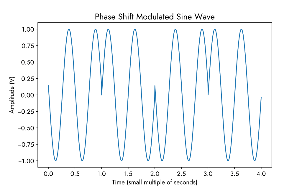
For example, 4-PSK refers to Phase Shift Key modulation with 4 separate symbols represented by 4 different phase shifts, with each symbol made up of 2 information bits: 00, 01, 10, 11.
4-PSK representing the sequence 1, 0, 1, 0:
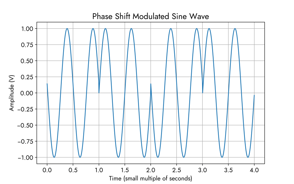
Including a grid on the plot helps see the separate symbols where each symbol spans a unit of time.
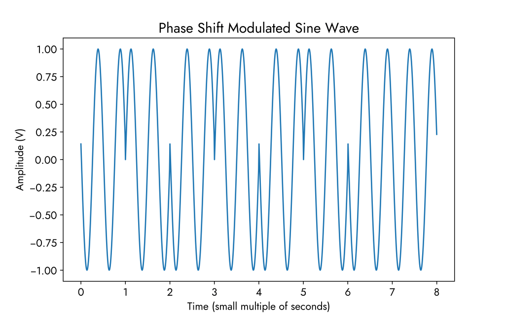
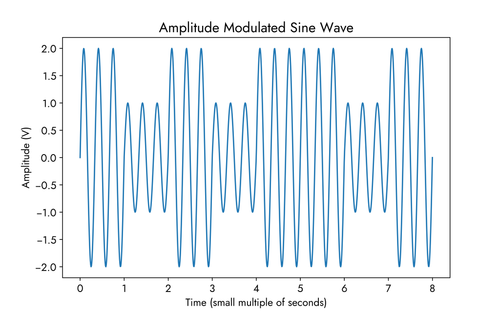
Next, an example of a waveform carrying 8 bits of information: 1, 0, 1, 0, 1, 0, 1, 1. Notice that the frequency remains the same since we still have two periods per second.
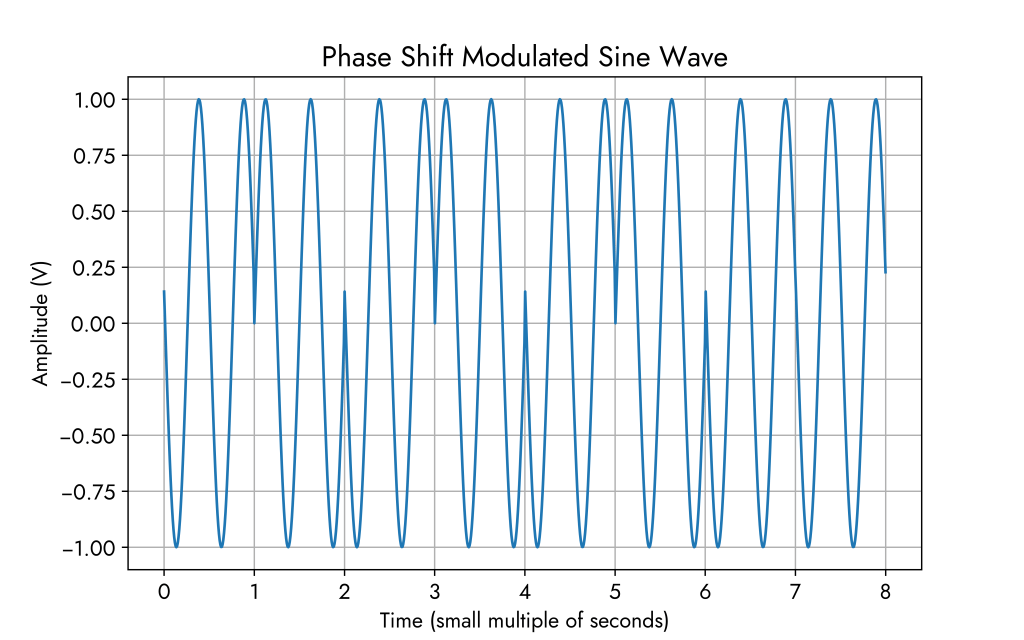
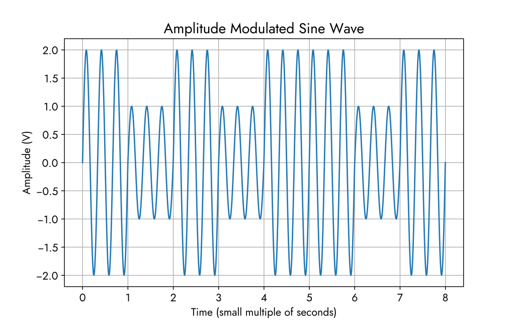
The same waveform with a grid on:
Amplitude Modulation (AM)
In AM transmissions, data symbols are distinguished by varying amplitudes as seen below.
With grid on:
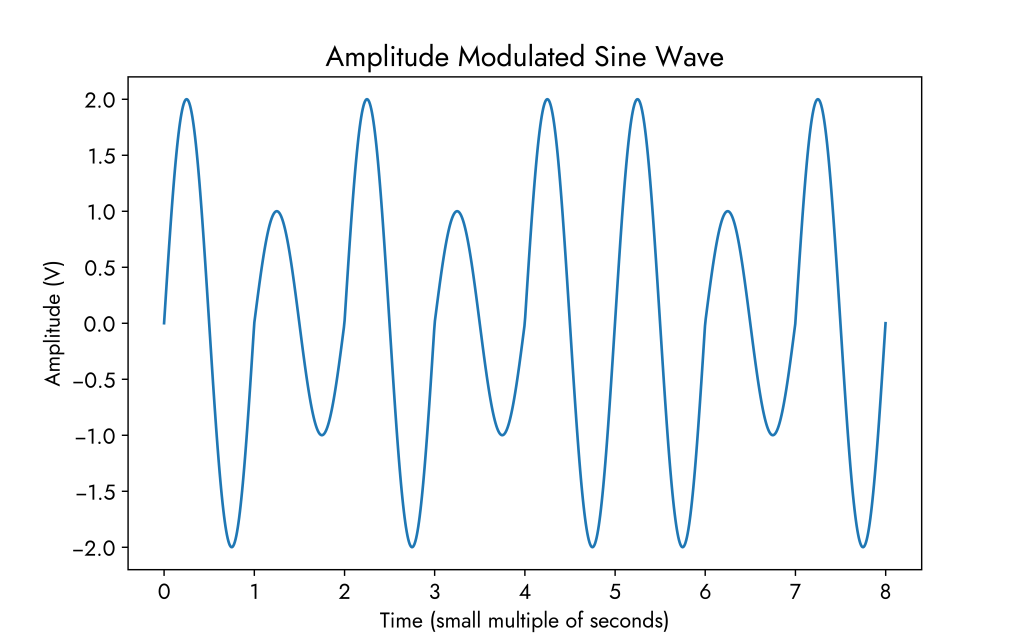
Decreasing the frequency to 1 Hz:
Constellation Diagrams
These diagrams are representations of sequences of waveforms in the complex plane, in other words – on an Argand diagram where the ‘In-Phase’ component is the real part and the ‘Quadrature’ component is the imaginary part of a point on the plane. A point’s coordinates are essentially the real and imaginary parts of the complex number. The magnitude of the complex number corresponds to the signal ampitude while its argument (angle from positive x-axis) represents the phase shift.
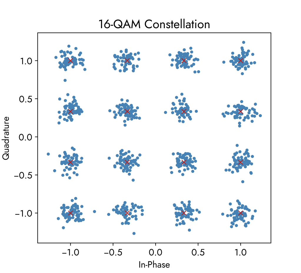
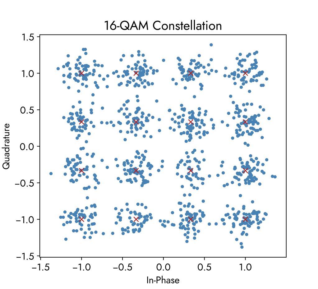
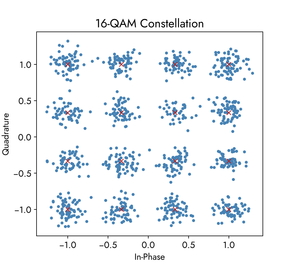
The visualisation below shows a 16-QAM constellation in which we can have 16 separate wave states with each state able to carry 4 bits of information. This simulation transmits 1000 data symbols and also adds in noise, resulting in a spread of amplitude and phase. Red crosses mark the exact theoretical positions the 16 symbols.
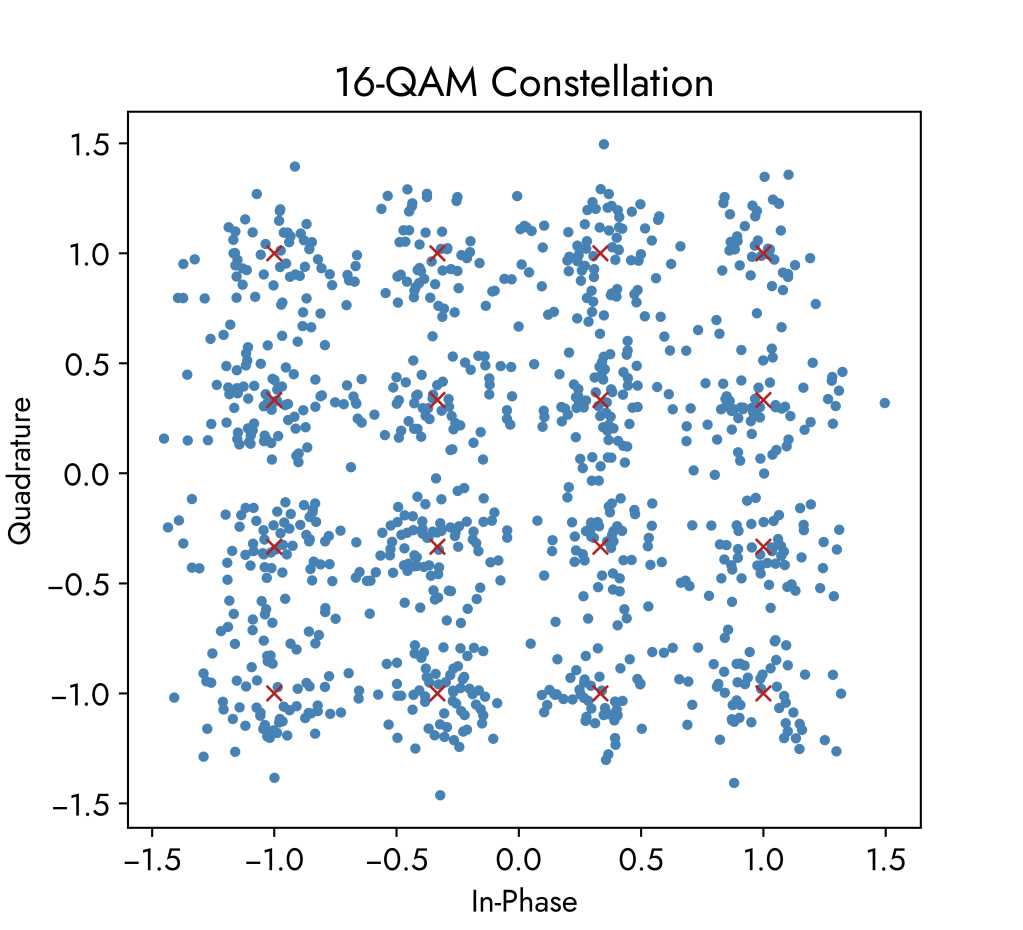
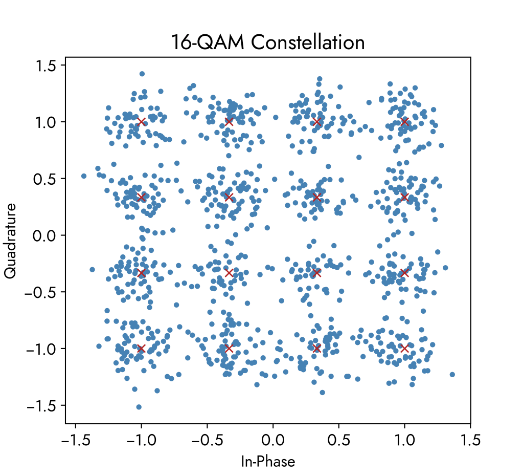
Swiping left through the constellation graphs shows the effects of increasing noise.
Noise is modelled as Additive White Gaussian Noise (AWGN) which is a basic model of a natural background noise signal that is added onto all transmitted information signals. Electronic noise is inevitable in communication systems as it is caused by natural processes such as temperature differences and acoustic noise and vibrations. In Gaussian Noise the amplitudes of the noise components follow a normal distribution with a variance that is usually small relative to the signal amplitude. These components are then added onto our information signal, hence the term ‘additive’.
Simulations use the noise levels in the table below that are all relative to the 1 Watt normalised power of the transmitted signal. Power normalisation helps keep the graph axis consistent when it comes to visualisation and also makes comparison easier.
| Noise Power (Watts) | Noise Power (dB) |
| 0.01 | -20 dB |
| 0.02 | -17 dB |
| 0.03 | -15.2 dB |
| 0.04 | -14 dB |
| 0.05 | -13 dB |
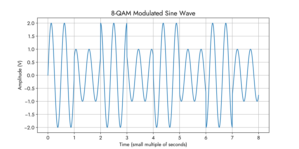
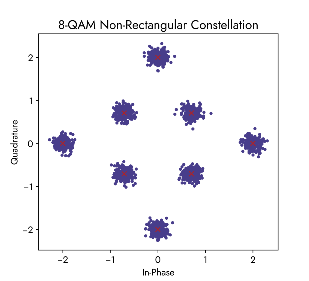
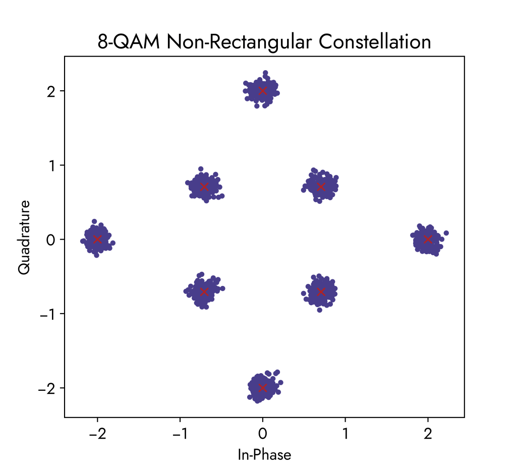
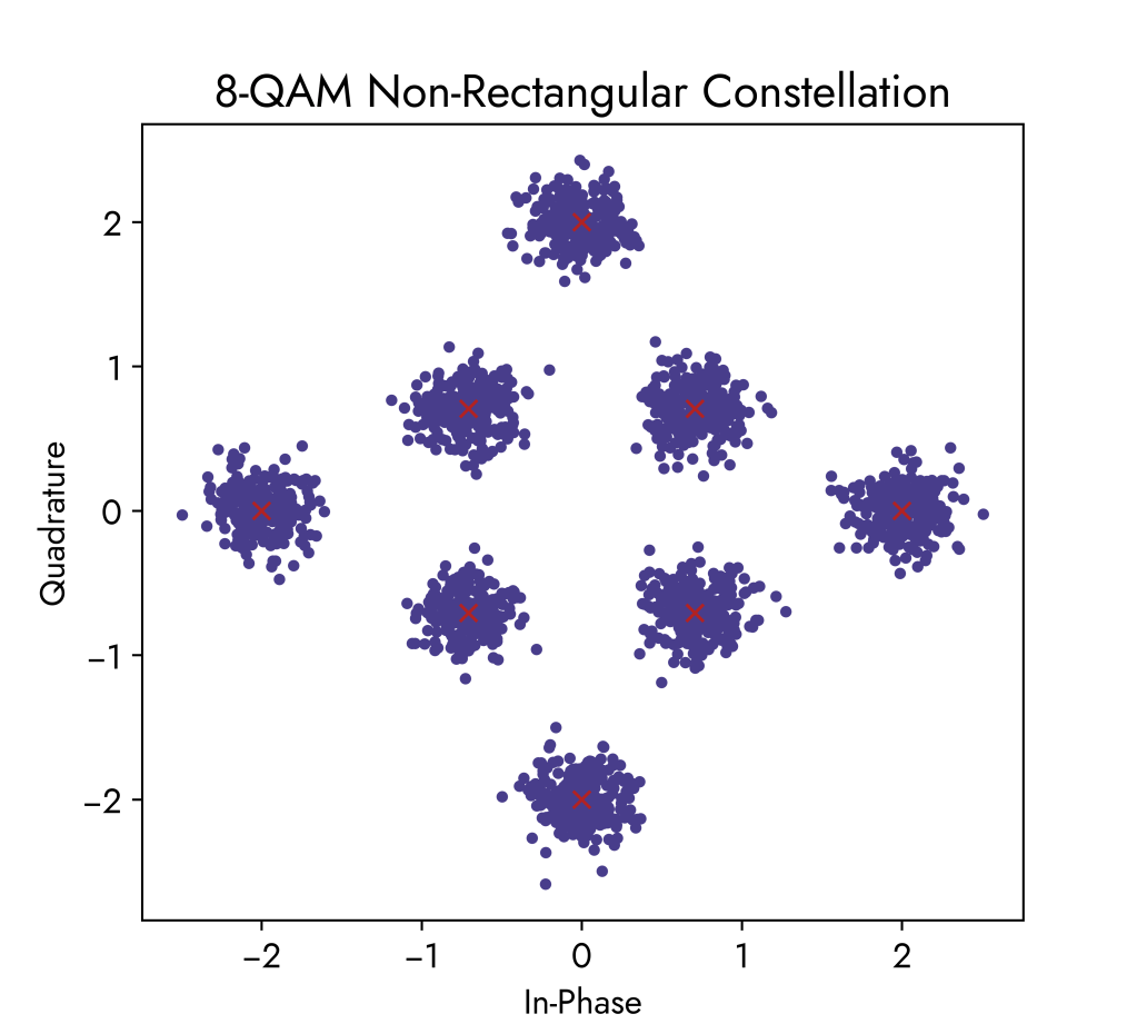
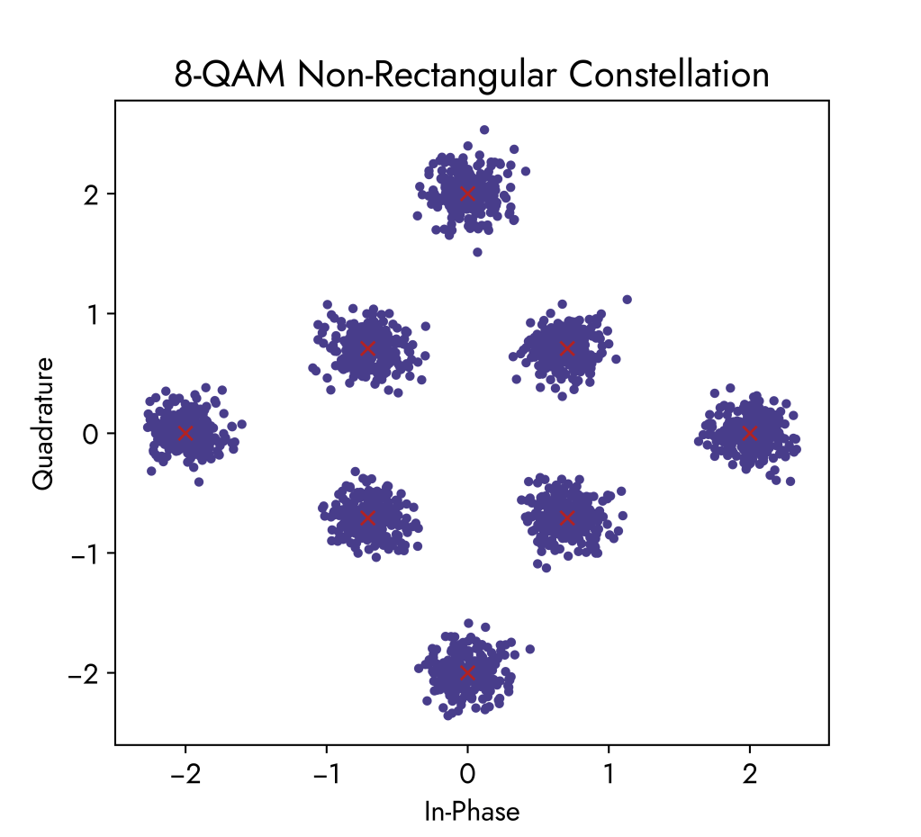
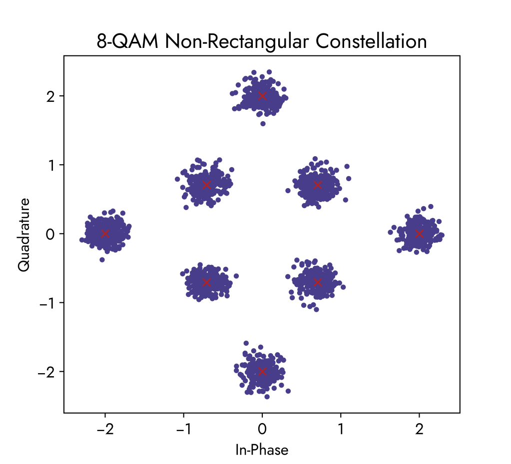
8-QAM (Non-Rectangular Constellation)
The 8-QAM constellations below use the same noise power increments as before. Comparing with the 16-QAM constellation, we can see that there is less likelihood of received symbols overlapping when there is high noise. Therefore, errors at the receiver are decreased since the points are not getting blended together.
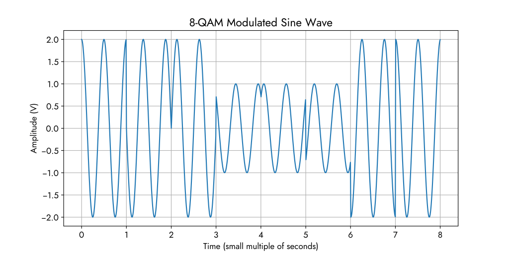
The below waveform corresponds to the 8-QAM constellation diagram. We can see that we have 8 different data symbols possible where each data symbol carries 3 informatiom bits because 23 = 8 and log2(8) = 3. Amplitude alternates between 1 and 2 (so not a power of 1 in this case) while the phase shifts in degrees are the following:
phase_shifts_deg = [0, 45, 90, 135, 180, 225, 270, 315]This sequence of symbols follows the 8-QAM constellation points in an anti-clockwise direction (counting up in 3-bit binary numbers to show all possible states in 8 symbols) but they do not necessarily need to be in this order.
Another 8-QAM waveform could be the following – representing a random sequence of 3-bit data symbols ‘010’, ‘100’, ‘000’, ‘011’, ‘001’, ‘111’, ‘110’, ‘010’.
QAM has become incredibly important and useful in many communication systems we rely on daily, ranging from our mobile phones and WiFi to TV and satellite communications.
Some of the underlying theory of modulation and signal processing is detailed by M. Lichtman in [1] and [2]. Programming techniques from the video lecture [3] were used for working with signals in Python including the ‘matplotlib’ and ‘numpy’ libraries.
Full Expandable Gallery
References
[1] M. Lichtman, “4. Digital Modulation,” PySDR: A Guide to SDR and DSP using Python. https://pysdr.org/content/digital_modulation.html (accessed 01/11/2024).
[2] M. Lichtman, “7. Noise and dB — PySDR: A Guide to SDR and DSP using Python,” pysdr.org. https://pysdr.org/content/noise.html (accessed 01/11/2024).
[3] “Representing Signals in Python (Sampling),” YouTube, Aug. 27, 2023. https://youtu.be/FDUJsATFZyI?si=FAjM3p2_b3dOn33L (accessed 01/11/2024).
