P5.js is an interesting JavaScript open-source library developed for programming dynamic graphical web applications. It offers a great deal of functionality for creating simulations or animations in the browser and is very similar to the processing.js library. The goal of this project is to build a new expanded version of the Fourier series simulation created by Daniel Shiffman on the Coding Train YouTube channel [1]. It features 5 additional simulations of common waveforms’ Fourier series representation. They may be helpful in visually understanding how Fourier series work. The number of terms can be adjusted with a slider below the canvas which varies how accurately a waveform is displayed.

Simulation available here: https://editor.p5js.org/czahariev/present/uTp9F7d3O
Background on the Fourier series
The Fourier series is a method of representing any periodic function as an infinite sum of weighted sinusoidal trigonometric functions. A periodic function is one in which its values are repeated over a regular time interval. In practice, a Fourier series is an approximation to the original function as only a finite number of terms are used. As the number of terms increases, the series representation gets closer and closer to the function. For most applications, about 10 to 20 terms provides a very accurate approximation as the series tends to converge very fast.
Trigonometric functions, on which the Fourier series is based, can be defined through circular motion as the coordinates of each point on a circle are related to the angle and radius through the equations and
where
is the radius and
is the angle (this can also be a paramter like time). Adding a new term to the series is equivalent to the addition of a new rotating circle in the simulation. In this case, radii act like vectors added together, with the y coordinate of the end of the resultant vector being the value of
. As every term in a Fourier series has its own amplitude and frequency, each new circle likewise has its own radius and angular frequency.
Finding the series expansion of a function is a matter of calculating the constants
and
. This can be done through the following standard integrals [2].
Where T is the period of the signal, is the angular frequency,
is a constant and
is a function of time. Notice that a0 is just the average value of the original function which acts as a vertical shift, or a DC component. Below is an example of finding the coefficients for a square wave with a period of 2, with no vertical offset. All the other waveforms’ series can be obtained with the same method and we will see how they are implemented in JavaScript later on.
As a rule, is always equal to 0 for odd functions. Conversely, an even function can only be made up of even sinusoids (cosine waves), so then
would be zero [2]. This square wave has no DC component, so
is also zero.
The mathematics behind the Fourier series was originally invented for solving both ordinary and partial differential equations. In physics and engineering, the Fourier series is useful for analysing discontinuous functions – for example signals modulated with binary phase shift keying in telecommunications. Another example is that if a triangular waveform is used as an input to an AC circuit, finding the Fourier series expansion means we can apply the principle of superposition to get the output or calculate unknowns such as impedances, voltages and currents [2, 3].
JavaScript program
At the start, the ‘setup()’ function defines the initial properties of the canvas area. In the ‘createCanvas’ function the dimensions are set to a width of 1000 px and a height of 400 px. P5.js contains some reserved variable names for specific purposes including the height and width variables used to calculate the ‘x’ and ‘y’ position variables. Before ‘setup’, all the variables are declared in the global scope so they can be used by every function. With P5, we can use ‘let’ or ‘var’ interchangeably [4].
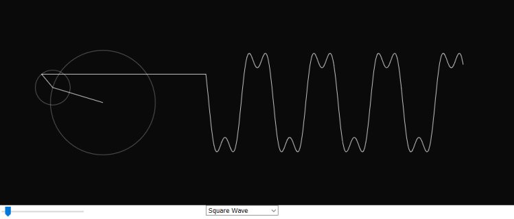
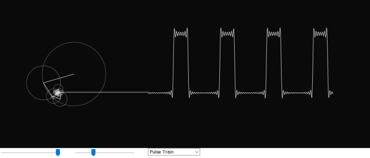
The ‘termSlider’ variable is assigned to a ‘createSlider’ function that sets up a slider input whose values range from 0 to 20 in steps of 1. The same thing is done for ‘dutyCycleSlider’ except the range is larger as it needs to cover values of 5% to 95% (0 to 100 would cause problems when graphing). To start with, the slider for the duty cycle input is hidden as it only needs to be shown for one of the waveforms.
Next, the ‘createSelect’ function creates a dropdown menu for selecting which waveform is shown. Again, the ‘position’ method specifies where it appears relative to the canvas, while the ‘option’ method simply adds a choice.
var time = 0;
var yArray = [];
var termSlider;
var dutyCycleSlider;
var DCLabel;
var sliderValue;
var phase;
var freq;
var radius;

function setup() {

    // Setting canvas dimensions and centering it
    var canvas = createCanvas(1000, 400);
    var x = (windowWidth - width) / 2;
    var y = (windowHeight - height) / 2 + 20;
    canvas.position(x, y);

    // Sets the number of terms in the Fourier series
    termSlider = createSlider(0, 20, 1);
    termSlider.position(x, y + height);

    let termLabel = createP('Number of terms (0 to 20)');
    termLabel.position(x - 290, y + height + 20);

    // Slider that sets the duty cycle of the pulse train
    dutyCycleSlider = createSlider(5, 95, 1);
    dutyCycleSlider.position(x + 200, y + height);
    dutyCycleSlider.hide();

    DCLabel = createP('Duty Cycle percentage');
    DCLabel.position(x - 80, y + height + 20);
    DCLabel.hide();

    // Dropdown menu for selecting a waveform
    dropdown = createSelect();
    dropdown.position(x + 400, y + height);
    dropdown.option('Square Wave');
    dropdown.option('Sawtooth Wave');
    dropdown.option('Rectified Sine Wave');
    dropdown.option('Triangular Wave');
    dropdown.option('AMI RZ Signal');
    dropdown.option('Pulse Train');

}
Calculating Fourier coefficients and circular motion coordinates
The ‘calculateSeries’ function does the majority of the heavy lifting in the program. It translates the Fourier series equations into JavaScript code. A variable ‘choice’ is assigned to the current option selected in the dropdown menu by the ‘value’ method. Then, the x and y coordinate variables are declared in the local scope of the function – they are different to the x and y seen in the setup function. In addition, the program needs to store the previous ‘x, y’ values, which is done in the ‘px’ and ‘py’ variables. They are necessary for centering each newly added circle on the circumference of the last circle and also for drawing all the radii.
The first ‘if-else’ statement checks whether the slider for the Pulse Train wave’s duty cycle needs to be displayed. Other waveforms don’t need this. A ‘for’ loop is used for the summation of terms in the series. On each iteration of the loop the code will work out a term of the series and add it to the previous term. This is repeated from i = 0 to the number of terms set through the slider input whose range is 0 to 20.
By calling ‘calculateSeries’ from ‘draw’ we are effectively creating a nested loop. Each time ‘calculateSeries’ is called, the ‘for’ loop runs to calculate the selected number of terms. It continuously updates the x and y values as it does so. Once the end is reached, the ‘unshift’ method appends the y coordinate needed for graphing to the beginning of ‘yArray’. The ‘beginShape’ function in P5 can draw any shape based on vertices given to it. To plot the waveforms, another loop is created and used to index ‘yArray’ until the end of this array. The ‘vertex’ function then plots ‘i’ versus the ith element of the array which is equivalent to the Fourier series value of .
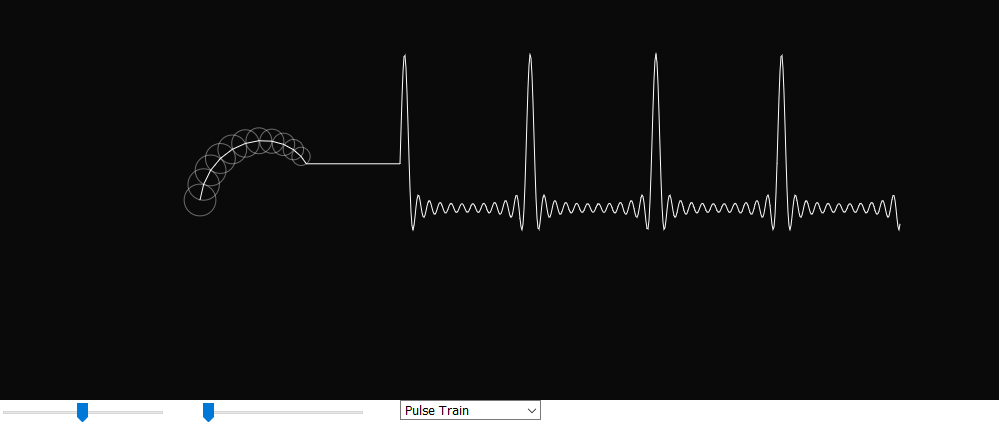
For example, if the slider is set to 2, for each draw loop, the ‘for’ loop below runs twice and two circles are drawn. The first one is centered at (0, 0) while the second one’s center is determined by the parametric equations, so it moves along the circumference of the first circle.
function calculateSeries() {

    let choice = dropdown.value();

    let x = 0;
    let y = 0;

    if (dropdown.value() == 'Pulse Train'){
        dutyCycleSlider.show();
        DCLabel.show();
    } else {
        dutyCycleSlider.hide();
        DCLabel.hide();
    }

    for (let i = 0; i <= termSlider.value(); i++) {

        /*
         Coefficients are calculated inside this loop.
         They are shown separately for clarity.
        */

        // Saving the last x and y values
        let px = x;
        let py = y;

        // Calculates points on a circle
        // Frequency and phase can vary
        x += radius * cos(freq * time + phase);
        y += radius * sin(freq * time + phase);

        stroke(255, 100);
        noFill();
        ellipse(px, py, radius*2);
        fill(255);
        stroke(255);
        line(px, py, x, y);
    }

    // Each y value is added to the start of the array
    yArray.unshift(y);

    translate(200, 0);
    line(x-200, y, 0, yArray[0]);
    beginShape();
    noFill();

    for (let i = 0; i < yArray.length; i++) {
        vertex(i, yArray[i]);
    }
    endShape();

}
Formulae for each waveform
Inside the ‘for’ loop, a series of ‘if-else if’ statements check which waveform is selected from the dropdown menu and then run the appropriate code. This is shown separately below for clarity. All the other Fourier series can be obtained with the same method as the square wave example seen earlier, although they can also be looked up in tables as the focus here is on the simulation rather than doing a lot of integration.
Below is a comparison of the Fourier series representation of each of the waveforms with the JavaScript code for calculating the coefficients. Anything that isn’t the sinusoidal function is factored out and combined in the ‘radius’ variable since this gives the value of the radius for each circle on the left side of the canvas [4, 5, 6].
When the Fourier series expansion involves a cosine, a phase shift of (or 90 degrees) is added as the ‘yArray’ values come from a sine function. This simply means we don’t have to repeat code with multiple arrays for different tasks.
Rectified Sine Wave
Here ‘j’ is declared as as a separate counter starting at 1 because starting at 0 results in incorrect plotting. The phase is set to half of pi since we need terms of cosine.
 if (choice == 'Rectified Sine Wave') {

            // In this case, a counter starting at 1 is needed
            let j = i + 1;

            n = 4*j*j - 1;
            freq = j;
            radius = 160 * (4/(n*PI));
            phase = HALF_PI;
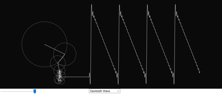
Sawtooth Wave
} else if (choice == 'Sawtooth Wave') {

             if(i % 2 == 0) {
                n = i + 1;
                freq = n;
            } else {
                n = -(i+1);
                freq = n;
            }
            phase = 0;
            radius = 80 * (4/(n*PI));
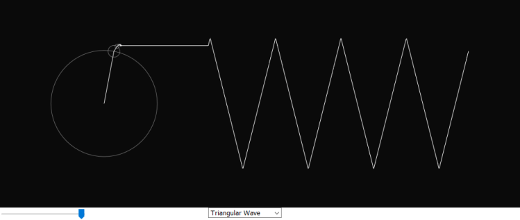
Triangular Wave
} else if (choice == 'Triangular Wave') {

            n = 8*pow(-1, (i+1));
            let den = PI * PI * (2*i+1) * (2*i+1);
            freq = 2*i + 1;
            radius = 126 * (n/(den));
            phase = 0;
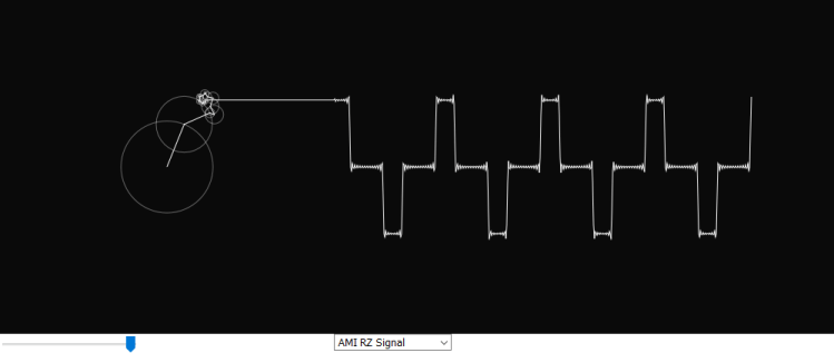
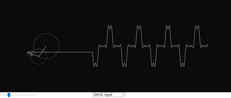
Alternate Mark Inversion Return to Zero Waveform
The variable names sometimes don’t match the ones in the formulae, which may be a bit confusing but here the n in the formula corresponds to i in the code below.
} else if (choice == 'AMI RZ Signal') {

            n = 2*i + 1;
            freq = n;
            radius = 80 * (4/(n*PI)) * cos(freq + phase);
            phase = TWO_PI;
Pulse Train Waveform
} else if (choice == 'Pulse Train') {

            n = i + 1;
            freq = n;
            let dc = 1 - (dutyCycleSlider.value()/100);
            radius = 80 * (4/(n*PI)) * sin(n*PI*dc);
            phase = HALF_PI;
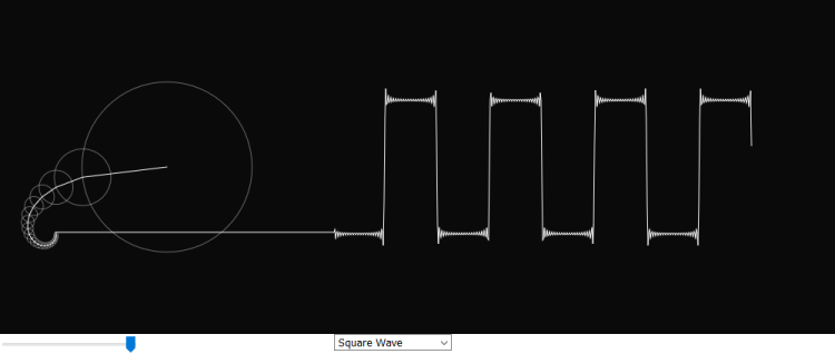
Square Wave
  } else {

            // A square wave signal shown as a default
            n = 2*i + 1;
            freq = n;
            radius = 80 * (4/(n*PI));
            phase = 0;
        }
Iterative control function
Finally, the ‘draw’ function works as a controller for the program. It is called repeatedly, so the drawings in the simulation are updated, creating the animation effect. The ‘time’ variable which starts off as zero increases by a step of 0.05 on every function call. It is then used in ‘calculateSeries’ for calculations. To make sure the program doesn’t use too much memory and slow down the browser, elements of ‘yArray’ are removed with the ‘pop’ method once its length reaches 500 elements. No more are needed to show the graph on the canvas.
function draw() {

    // Shifts objects 200 px down and to the right
    translate(200, 200);
    background(10);

    calculateSeries();
    // Increment time by 0.05 each time draw is called
    // Changing the sign reverses the direction of rotation
    time += 0.05;

    // Remove elements from array after a length of 500
    // Prevents program from slowing down
    if (yArray.length > 500) {
        yArray.pop();

    }

}
Thanks for reading!
by Constantine Zahariev
References
[1] “Coding Challenge #125: Fourier Series”, 2018. [Online]. Available: https://www.youtube.com/watch?v=Mm2eYfj0SgA&feature=emb_title. [Accessed: 02- March- 2020].
[2] M. van Biezen, “Ilectureonline”, Ilectureonline.com, 2020. [Online]. Available: http://www.ilectureonline.com/lectures/subject/ENGINEERING/28/260. [Accessed: 10- Mar- 2020].
[3] “Applications of Fourier Series to Differential Equations”, Math24, 2020. [Online]. Available: https://www.math24.net/fourier-series-applications-differential-equations/. [Accessed: 20- Mar- 2020].
[4] “Reference | p5.js”, P5js.org, 2020. [Online]. Available: https://p5js.org/reference/. [Accessed: 14- Mar- 2020].
[5] “The Fourier Series of Selected Waveforms”, web.calpoly.edu, 2020. [Online]. Available: https://web.calpoly.edu/~fowen/me318/FourierSeriesTable.pdf. [Accessed: 16- Mar- 2020].
[6] S. Smith, “The Fourier Series”, Dspguide.com, 2020. [Online]. Available: https://www.dspguide.com/ch13/4.htm. [Accessed: 08- Mar- 2020].
